The 1-2% Rule Foundations
Nearly every serious crypto trader starts with the golden rule: never risk more than 1–2% of your total account on a single trade. This principle isn’t pulled from thin air – it’s a statistical safety net against ruin. When you risk a tiny, fixed fraction, a string of losses can’t wipe you out. Even after ten consecutive losing trades at 2% risk, you’d still retain about 81% of your original capital (1 – 0.02)^10 ≈ 0.817). Contrast that with aggressive 10% bets, where ten losses leave you with just 35%, and the math becomes stark.
Why 1–2% Became the Gold Standard
The 1–2% rule originates from professional risk managers and veteran traders who understand that survival is the first step to profitability. It’s deeply rooted in the concept of the risk of ruin – the probability that your account will hit zero before turning a profit. By capping risk per trade, you effectively flatten that curve, making ruin highly unlikely even during severe drawdown periods. In crypto’s volatile markets, where double-digit swings are common, this anchor is even more critical.
The Problem with Fixed Fractional Risk
While fixed fractional risk protects capital, it treats every signal identically. But not all trade setups are created equal. A setup backed by converging on-chain data, heavy whale accumulation, and bullish derivatives metrics is far more likely to succeed than a quick scalp based on a single moving-average crossover. Blindly risking 1% on both ignores the quality of your signal – and leaves potential profit on the table for your strongest ideas. This is where a position sizing confidence score transforms static risk into intelligent, dynamic sizing.
Introducing Confidence-Adjusted Risk
Confidence-adjusted risk means you start with a base risk percentage – say 1% – and scale it up or down based on the strength of your trade signal. If a high-confidence signal surfaces, you might risk 1.5% of the account. For a mediocre signal, you risk only 0.5%. The result is that your strongest convictions compound faster while weak ideas barely dent your equity. This approach mirrors professional fund management, where capital is allocated asymmetrically toward the highest-probability trades.
Calculating Position Size from Risk %
The Basic Position Size Formula
Before you can scale by confidence, you must master the core position-sizing calculation. The classic formula is:
Position Size = (Account Equity × Risk %) / (Entry Price – Stop-Loss Price)
Suppose you have a $10,000 account, you’re willing to risk 1% ($100), and you plan to enter BTC at $65,000 with a stop at $63,700 (a $1,300 risk per coin). Your position size would be $100 / $1,300 ≈ 0.0769 BTC. That’s roughly 0.077 BTC, a straightforward calculation. But this assumes every trade deserves the same 1% – which it doesn’t.
Accounting for Leverage
If you trade perpetual futures, the same dollar risk still applies, but leverage changes the notional value. For example, with 10x leverage, a 0.077 BTC position has a notional value of 0.77 BTC. The risk remains $100 because your stop-loss limits the loss to the predetermined amount. Always calculate position size from dollar risk, not leverage. Leverage simply lets you deploy less margin for the same exposure; it does not alter the risk-first logic.
From Fixed Risk to Dynamic Risk
Once you’ve internalized the formula, the next evolution is tying your risk % to a position sizing confidence score. Instead of a flat 1%, you multiply that base by a confidence multiplier. For instance:
- Base risk = 1% of account
- Confidence multiplier = 1.5 (for a HIGH confidence signal)
- Adjusted risk = 1.5%
Now your position size becomes $150 / $1,300 ≈ 0.1154 BTC. The math is simple, but the real craft lies in systematically generating that confidence score. That’s where tools like Smart Money API fill the gap – they fuse derivatives data, on-chain flows, whale wallet activity, and macro signals into one unified composite score, giving you an objective confidence tier you can plug directly into your spreadsheet or calculator.
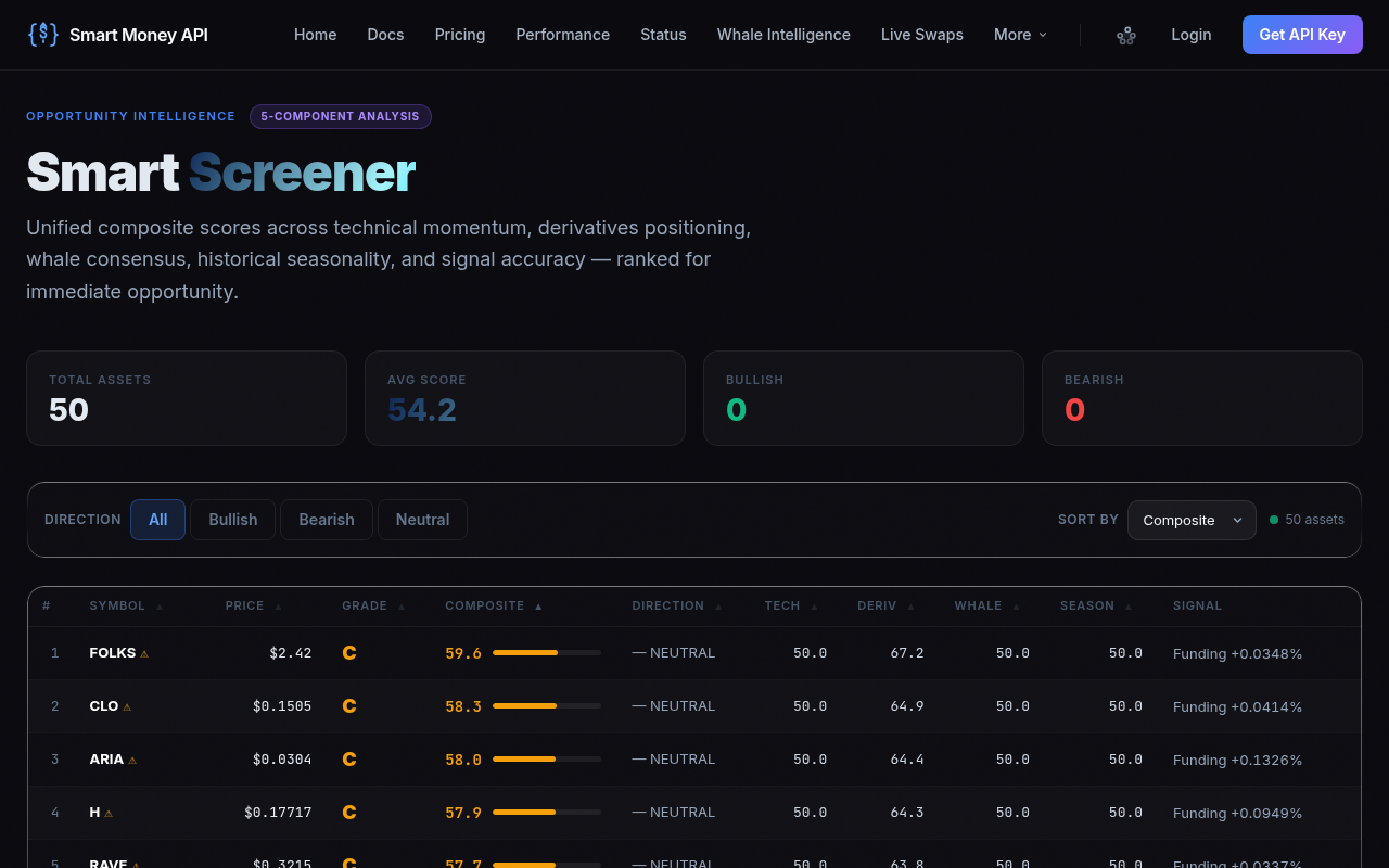
For a quick, manual calculation without any external data, you can still use a trusted tool like the CryptoCalcs Position Size Calculator. It handles the arithmetic, so you just input your risk and stop distance. But to make that calculator truly powerful, you need a confidence number to feed into it.
Defining Confidence Score Tiers
Building a Confidence Score Framework
A robust confidence score quantifies the strength of your trade thesis on a 0–1 scale (or 0–100). It aggregates multiple data layers – technical setup, on-chain signals, macro sentiment, order flow – into a single number. For instance, a score of 0.8–1.0 might mean the signal is extremely high probability, while 0.3–0.5 suggests the edge is marginal. The challenge is how to source such a score without building your own complex model. APIs like Smart Money API’s /v1/confirm endpoint solve this by processing real-time data and outputting a composite score and a confidence tier.
GET /v1/confirm?symbol=BTC&direction=long
{
  "composite": 0.74,
  "confidence": "HIGH",
  "action": "CONFIRM",
  "size_mult": 1.5,
  "deriv_score": 0.81,
  "onchain_score": 0.68,
  "whale_score": 0.73
}
In this example, the API returns a HIGH confidence level, a composite score of 0.74, and even suggests a size_mult of 1.5 – meaning you could multiply your base risk by 1.5 for this trade. This takes the guesswork out of defining tiers.
Example Tier Thresholds
If you decide to build your own tiered system, you might set thresholds like this:
| Confidence Tier | Score Range | Risk Multiplier |
|---|---|---|
| HIGH | 0.70 – 1.00 | 1.50x |
| MEDIUM | 0.40 – 0.69 | 1.00x |
| LOW | 0.00 – 0.39 | 0.50x |
These multipliers mean a HIGH-confidence trade would risk 1.5% on a base 1% account risk; a LOW-confidence signal risks only 0.5%. The exact thresholds depend on your backtesting, but the principle holds: allocate more capital to stronger signals.
Assigning Risk Multipliers Consistently
Consistency is key. Do not arbitrarily assign multipliers based on gut feeling. Use a well-defined set of criteria – perhaps the number of confirming indicators, the alignment of volume, or a composite algorithmic score. The beauty of Smart Money API is that it standardizes this process. Its composite score is derived from three pillars: derivatives sentiment (deriv_score), on-chain activity (onchain_score), and whale wallet movements (whale_score). When all three are bullish and the composite > 0.7, the multiplier is 1.5. This objectivity removes emotional bias and ensures you follow the same risk-scaling rules every time.
High/Medium/Low Confidence Examples
Let’s walk through three concrete scenarios on a $10,000 account with a base risk of 1% and a BTC setup where the entry is $65,000, stop-loss at $63,500 (risk per coin $1,500).
HIGH Confidence Trade
Confidence composite = 0.82 (HIGH). Multiplier = 1.5 → risk = 1.5% × $10,000 = $150. Position size = $150 / $1,500 = 0.10 BTC. The stronger conviction gets 50% more capital at risk, maximizing return potential when the edge is sharp.
MEDIUM Confidence Trade
Composite = 0.55 (MEDIUM). Multiplier = 1.0 → risk = 1% × $10,000 = $100. Position size = $100 / $1,500 = 0.0667 BTC. The standard bet for a decent, but not exceptional, signal.
LOW Confidence Trade
Composite = 0.32 (LOW). Multiplier = 0.5 → risk = 0.5% × $10,000 = $50. Position size = $50 / $1,500 = 0.0333 BTC. Even if the trade fails, the damage is half the usual amount, preserving capital for better opportunities.
This gradient of sizing aligns capital exposure with the probability of success. Over time, you tilt your bet distribution toward high-probability events – the very mechanism professional quant funds use to outperform.
Kelly Criterion & Bet Sizing
Understanding the Kelly Formula
The Kelly Criterion is a mathematical formula that calculates the optimal fraction of your bankroll to bet to maximize long-term growth. The classic formula for a binary outcome is:
f* = (bp – q) / b
where:
- b = net odds received on the bet (win/loss ratio, e.g., if you stand to win $2 for every $1 risked, b=2)
- p = probability of winning
- q = probability of losing (1 – p)
If your signal has a 60% win rate (p=0.6) and your average reward-to-risk is 2:1 (b=2), then f* = (2×0.6 – 0.4)/2 = (1.2 – 0.4)/2 = 0.4. The Kelly suggests risking 40% of the account – far too much for most traders. That’s why fractional Kelly (half-Kelly, quarter-Kelly) is used to tame volatility.
Adapting Kelly for Crypto
In crypto, win rates and reward-to-risk ratios are rarely stationary. Moreover, the heavy tail risk of sudden crashes makes full Kelly dangerously aggressive. Many professional traders use half-Kelly or even quarter-Kelly, turning that 40% into 20% or 10%—still aggressive relative to the 1–2% rule, but mathematically optimal if your estimates are accurate. The real challenge is accurately estimating p and b. A confidence score can feed those estimates. For instance, a HIGH confidence trade with a composite of 0.74 might imply a win probability of 0.62 (based on historical backtests), turning Kelly into a dynamic, confidence-driven number.
Confidence-Adjusted Kelly
Instead of a static win probability, you can map your confidence score directly to an estimated edge. If your score is 0.8, you might assign p=0.65; if 0.5, p=0.55. Then use fractional Kelly to calculate the risk fraction. For example:
Half Kelly with p=0.65, b=2 → f* full = (2×0.65 – 0.35)/2 = 0.475; half = 0.2375. That 23.75% of the account is still way too high for most, so you’d cap it at, say, 3% maximum. The point is that the Kelly framework provides a logical, confidence-driven bet size, while a hard cap keeps ruin in check. A risk management calculator can help you simulate how different Kelly fractions affect your equity curve and drawdowns.
Account Curve Management
Position sizing doesn’t operate in a vacuum – your equity curve tells the story of how well your strategy is performing. A healthy equity curve trends upward with shallow, swift drawdowns. When it veers off course, your sizing rules should adapt. This is where dynamic position sizing based on recent performance adds a second layer of protection.
Using the Equity Curve as Feedback
Implement a simple rule: after a streak of, say, three consecutive losing trades, reduce your base risk by 20–30%. Conversely, after a winning streak, you could gradually increase base risk up to a ceiling. This anti-martingale approach ensures you press your edge when the market is cooperating and pull back when it isn’t. Pair this with confidence scoring, and you have a two-dimensional sizing system: confidence adjusts per trade, equity curve adjusts the base risk fraction globally.
Drawdown Thresholds
Set hard drawdown limits. For example, if your account drawdown exceeds 15% from the peak, cut all risk multipliers in half until you recover to within 10% of the peak. This rule prevents emotional revenge trading and enforces a cooling-off period. Many successful traders combine this with a confidence-score floor: when in drawdown, only take trades with a confidence score above 0.75. The result is that during rough patches, you’re only committing capital to the very best opportunities – a natural survival mechanism.
Dynamic Scaling During Drawdown
Drawdowns are inevitable, but how you size positions during them determines whether you recover or spiral. The confidence-score system must be flexible enough to tighten up when losses mount. Think of your sizing algorithm as a thermostat: when the account gets too hot (winning), you can raise the temperature slightly; when it cools (losing), you dial it down.
The Drawdown Scaling Formula
One approach: Adjusted Risk % = Base Risk% × Confidence Multiplier × Drawdown Multiplier. The drawdown multiplier could be 1.0 when drawdown is below 10%, 0.8 between 10–20%, and 0.5 above 20%. So, a HIGH confidence trade (multiplier 1.5) during a 15% drawdown would have an effective risk of 1% × 1.5 × 0.8 = 1.2% instead of the normal 1.5%. This automatic reduction fights the gambler’s fallacy and keeps your account alive.
Psychological Edge of Rule-Based Scaling
Knowing there’s a system in place that shrinks position sizes when you’re down removes the panic that leads to impulsive decisions. Instead of pulling the plug entirely, you just trade smaller, high-confidence setups. Over time, this discipline smooths the equity curve and instills a long-term mindset. Combined with a robust position sizing confidence score, it transforms your trading from reactive to pre-planned, almost mechanical.
Building Your Position Sizing Sheet
All of this theory becomes actionable when you build a simple position sizing spreadsheet or use a calculator that accepts risk multipliers. Here’s a step-by-step guide to creating your own dynamic sizing template:
Step 1: Input Parameters
Columns: Account Balance, Base Risk %, Current Drawdown %, Drawdown Multiplier (lookup table), Confidence Score, Confidence Tier, Risk Multiplier, Entry Price, Stop-Loss Price, Calculated Position Size.
Step 2: Lookup Tables
Use VLOOKUP or INDEX/MATCH to automatically assign the confidence multiplier based on your tier thresholds (like the table earlier). Similarly, map drawdown % to a drawdown multiplier.
Step 3: Formula
Adjusted Risk Amount = Account Balance × Base Risk % × Confidence Multiplier × Drawdown Multiplier. Then Position Size (units) = Adjusted Risk Amount / (Entry – Stop). This formula handles both spot and futures (just keep leverage separate).
Step 4: Pull Confidence Scores Automatically
This is where Smart Money API’s endpoint can feed directly into your sheet via a simple API call or connector. The size_mult value from the response can replace your manual confidence multiplier, ensuring your sizing always mirrors the latest composite intelligence. Free tier access lets you test this integration without upfront cost – simply grab your API key and start weaving real-time confidence data into your decision flow.
Step 5: Review and Refine
Backtest your sizing rules over historical data. See how the dynamic approach would have performed versus fixed 1% risk. Adjust multipliers and drawdown rules until the equity curve looks robust. Use the CryptoCalcs Position Size Calculator as a sanity check for individual trades when you’re not at your spreadsheet.
Start Sizing with Confidence Today
Mastering position sizing confidence score techniques can be the single biggest edge separating consistent traders from gamblers. By starting with a rock-solid 1–2% risk foundation, then layering on confidence-based multipliers, Kelly-informed adjustments, and drawdown-aware scaling, you build a capital-preservation engine that lets your winners run while choking off losers. The key is to systematize the confidence part – don’t rely on hunches. Leverage a composite scoring tool like Smart Money API, which fuses derivatives, on-chain, whale, and macro data into an objective confidence number, and even suggests the exact size multiplier for each trade. Integrate it with the calculators and spreadsheets you’ve built using the guidance above, and you’ll be trading with a professional-grade, risk-first framework. Ready to put dynamic sizing to work? Sign up for a free API key at Smart Money API and start receiving real confidence scores in your next trading session.